Carl Friedrich Gauss (1777–1855) was not only the prince of mathematicians, but also an applied mathematician who contributed to the development of the least squares method, numerical solutions of systems of linear equations, numerical solutions of integrals, the theory of interpolation, the Fast Fourier Transform (FFT), systems of ordinary differential equations, and more. He was also a mathematical physicist and a talented experimenter who conducted research in astronomy, geodesy, and geomagnetism [1, 2, 4, 6, 8]. In this study, we are interested in Gauss’s work on the terrestrial magnetic field. He was the first to model mathematically the magnetic field at the surface of the Earth, and to find numerical results. His model proved to be the most ambitious project of applied mathematics of its time. It is a perfect example of Joseph Fourier’s view of natural philosophy: “Profound study of nature is the most fertile source of mathematical discoveries” [3, p. 7]. However, this particular contribution by Gauss has been largely overlooked by the historians of mathematics, although it has been noted by geophysicists.

Erroneous explanations of the terrestrial magnetic field had existed for centuries. Christopher Columbus believed that the Polar star attracts a magnetic needle. Others thought that a magnetic mountain exists in the Arctic. William Gilbert, the physician of Queen Elizabeth I, destroyed all previous hypotheses when in 1600 he published De Magnete, theorizing that the Earth is a gigantic magnet with a north pole and a south pole.

Although Gauss became interested in the Earth’s magnetic field by 1803, it was not until 1839 that he published “Allgemeine Theorie des Erdmagnetismus” (on the mathematical modeling of the Earth‘s magnetic field). This appeared in a very obscure journal [5]—a fact that may help explain the historians’ neglect. Gauss examined William Gilbert’s hypothesis that the Earth is a magnet, and he further postulated that the magnetic potential obeys Laplace’s equation at the surface of the Earth as well as outside of the Earth. Gauss thus needed to solve the Laplace equation in spherical coordinates for a heterogeneous spherical terrestrial surface. Therefore, he required a magnetic map as a boundary condition at the surface of the Earth. Unfortunately for Gauss, the magnetic potential was not measurable. Only the components of the magnetic field were observable. The model is [6]:

\nabla^2V=0, \quad V(r\to +\infty) = 0,\quad {\partial V \over \partial r}(a, \theta, \phi) = Z,{1 \over r} {\partial V \over \partial \theta}(a,\theta,\phi)=X, \quad-{1\over r\sin\theta}{\partial V\over \partial \phi}(a,\theta,\phi)=Y,V(r,\theta,\phi+2\pi)=V(r,\theta,\phi).

Here V  is the potential,  r the radial distance, and a the earth’s radius. Therefore the declination is given by D=\arctan(Y/X), the inclination will be I=\arctan(Z/H) and the horizontal intensity is H=\sqrt{X^2+Y^2}.

Gauss used the method of separation of variables for the Laplace equation. He wrote the equation for the spherical harmonics, the formula to obtain the associated Legendre polynomials P_n^m, and arrived directly—without any explanations or references—at the correct solution in the form of a series of trigonometric functions and associated Legendre polynomials:

Y^{(n)}=g^{n,0}P^{n,0}+(g^{n,1}\cos\phi + h^{n,1}\sin\phi)P^{n,1} + (g^{n,2}\cos2\phi + h^{n,2}\sin2\phi)P^{n,2}+\cdots\quad +(g^{n,n}\cos n\phi + h^{n,n}\sin n\phi)P^{n,n}.

This equation represents fundamental progress over Legendre’s and Laplace’s 18^th-century results on the theory of gravitation. The coefficients g and h came to be called the Gauss coefficients. In modern notation, we have for the complete series of the potential [5]:
V(r,\theta,\phi) = a \sum_{n=0}^N \left({a\over r}\right)^{n+1}\sum_{m=0}^n P_n^m(\theta)[g_n^m\cos m\phi + h_n^m \sin m\phi].

Gauss limited himself to N = 4, or 24 Gauss coefficients for the derivatives of the potential. He already had observations from magnetic stations all around the terrestrial globe. By a technique of interpolation, he brought back the information to the nodes of a grid where the increments of \theta and \phi are constant [5, pp. 631–632]—creating one of the first examples of tessellation! This technique of bringing the information to the nodes of a grid is now called an objective analysis. Gauss selected 12 nodes on each of seven circles of latitude, for a total of 84 nodes. He then decomposed the problem by working from the colatitudes \theta = constant, and by doing a harmonic analysis. For example, he had:

X = \sum_{n=1}^4 \sum_{m=0}^n (g_n^m \cos m\phi + h_n^m \sin m\phi) {dP_n^m\over d\theta}, \quad\rm{i.e.,}\quad X=\sum_{m=0}^4(\alpha_{mx}\cos m\phi + \beta_{mx}\sin m\phi).

Consequently, he calculated nine Fourier coefficients \alpha_m,\beta_m per circle of latitude. In \alpha_{mx}, the subscript x refers to the component X of the magnetic field. These calculations had to be repeated for the seven circles of latitude, for a total of 63 coefficients. But he had to do the computations for the three components of the magnetic field, for an overall total of 63 \times 3 = 189 coefficients. By identification, he had [4]:

\begin{Bmatrix}\alpha_m \\ \\ \beta_{mx}\end{Bmatrix} =\sum_{n=m}^4 \begin{Bmatrix}g_n^m\\ \\h_n^m\end{Bmatrix}{dP_n^m(\theta) \over d\theta}.

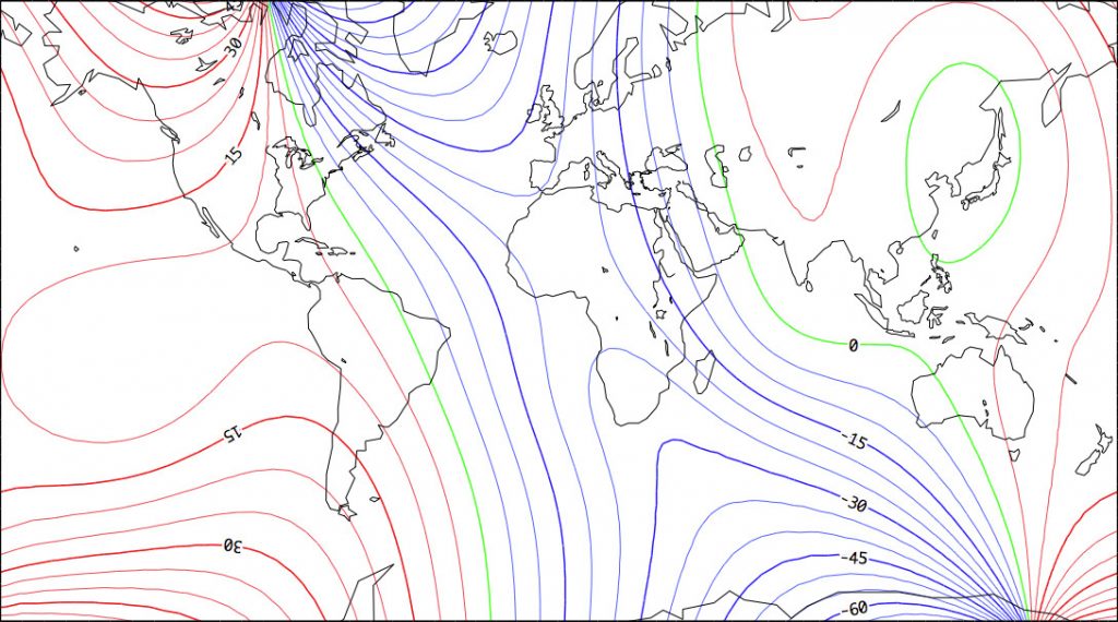
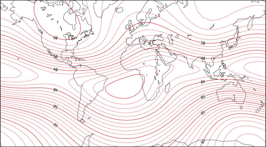
Gauss used the 189 values to solve by least squares these systems of equations in order to find the 24 Gauss coefficients. In Figures 1 and 2 we have recreated, with a computer, Gauss’s model and his results for the declination and the total intensity for the year 1835. His map of the intensity corresponds well to modern numerical results.

In conclusion, Gauss’s memoir of 1839, by using spherical harmonics, gave a mathematical form to Gilbert’s hypothesis. It was also a major contribution to applied mathematics. Let us quote James Clerk Maxwell, who wrote in 1873 [7, p. viii]:

Gauss, as a member of the German Magnetic Union, brought his powerful intellect to bear on the theory of magnetism, and on the methods of observing it, and not only added greatly to our knowledge of the theory of attractions, but reconstructed the whole magnetic science as regards the instruments used, the methods of observation, and the calculation of the results, so that his memoirs on Terrestrial Magnetism may be taken as models of physical research by all those who are engaged in the measurement of any of the forces in nature.

Geomagnetism remains a very active field of observation and theory, not least for its continuing utility for orientation and navigation, but also due to interest in ongoing changes within the Earth. The wandering of the magnetic poles over recent decades is one example, and outside the scope of this article, but it is worth noting that geomagnetic field data continue to be assimilated and distributed in the form of spherical harmonic coefficients, so that creating any map from historical or modern data involves tables of harmonic coefficients in the manner that Gauss began.

The International Geomagnetic Reference Field (IGRF) presents its model using spherical harmonics of degree and order 13. NOAA also has a series of models extending in some cases to degree and order 720. The terrestrial and lunar gravitational fields are reported and modelled using spherical harmonics, as are such diverse data as the cosmic microwave background. Gauss was visionary in his identification and application of a methodology critical to so many modern endeavours.

Roger Godard is an emeritus professor at Royal Military College, Kingston, Ontario, who has contributed regularly to CSHPM since 1991. John de Boer is a retired Major from the Department of National Defence and a professor at RMC. His field is mainly numerical simulations of auroral events and mathematical physics.